Resources
 Part of the Oxford Instruments Group
Expand
Collapse
Part of the Oxford Instruments Group
Application Notes
Author: Andrew P. Carpenter
Published: 01 Mar 2025 · Last updated: 24 Mar 2025
Spectroscopy provides a powerful means to explore the atomic and molecular world through absorption and emission spectroscopy, nonlinear spectroscopy, and many more spectroscopic methods. In some cases, the spectroscopic method being used to monitor an evolving system’s dynamics could benefit from having a camera possessing frame rate capabilities faster than the evolution of the chemical system being studied. The challenge, from a detection point of view, is how to preserve sensitivity while increasing speed since increases in the readout rate of a scientific camera lead to increases in the noise floor.
In this application note we highlight the application of one of the technological advantages of scientific CMOS (sCMOS) cameras, its ability to accommodate high acquisition rates, towards spectroscopic experiments. First introduced in 2009 sCMOS cameras are notable for their increase in acquisition speed, relative to CCD cameras, while being able to maintain a low noise floor. Much of the early adopters of these cameras were scientists interested in faster imaging cameras for use in areas such as live cell imaging or adaptive optics. However, in recent years there has been an uptick in interest for faster spectroscopy cameras and sCMOS camera technology is poised to be an excellent fit.
In this simple demonstration we measure the fast color transition in an RGB LED emission. This color change takes place over the course of milliseconds and we show how an sCMOS camera mounted onto a spectrograph can be used to monitor the full transition with sub-millisecond time resolution. While this experimental set-up is relatively simple, it highlights how an sCMOS camera can be used for fast spectral acquisitions, exceeding 1 kHz, and can be generalized to many spectroscopic methodologies.
For this work we measured the emission from an RGB LED using a Kymera 193i spectrograph and ZL41 Wave sCMOS camera (Figure 1). The RGB LED, hereafter referred to as the LED, has three different color channels (red, green, and blue) that are each controlled independently, allowing for the emitted color to be rapidly changed. An Arduino is used to execute changes to LED emission by adjusting the voltage supplied to each color channel.
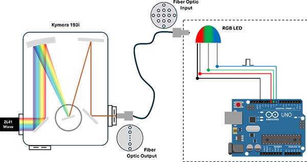
Figure 1. Overview of the experimental setup including a description of how the LED was connected to the Arduino, a general illustration of the input/output of the fiber optic cable, and Czerny-Turner geometry of the Kymera 193 spectrograph.
The Kymera 193i spectrograph was configured with a 600 l/mm diffraction grating. When matched with the ZL41 Wave 4.2 the resolution and bandpass of this system is 0.5 nm and 105.5 nm, respectively. The ZL41 Wave 4.2 was connected to the computer using a USB 3.0 cable. For all spectral measurements the LED and Arduino were placed in a light tight box. LED emission was collected using a fiber optic cable containing 19 cores with 100 µm diameters that is vertically stacked at the exit to optimize the collection for spectroscopic purposes. All experiments were ran using Andor’s Solis software.
LED emission was first characterized in the steady state using an exposure time of five seconds. The emission of individual color channels was characterized at fixed diffraction grating angles. To characterize the individual channels, the voltage applied to the off-color channels was set to zero and the voltage applied to the channel of interest was held at a fixed value. The “white light” spectrum, where all colors are turned on, was characterized at multiple grating positions and stitched together using the Step-n-Glue function in Solis (Figure 2). To generate the white-light spectrum the voltages applied to each channel were held at the same fixed value. The red, green, and blue channels are shown to have emission spectra peaked around 630 nm, 520 nm, and 470 nm, respectively. Overlaying the individual colors with the white light spectrum it is clear the white light spectrum is simply the combination of the three different individual colors, as would be expected.
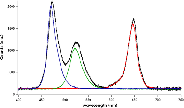
Figure 2. Steady state spectra of the three individual color channels (blue, green, and red) and the white light spectrum, when all three colors were turned on simultaneously.
To illustrate the use of an sCMOS to monitor fast dynamical systems, we measured a fast color change in LED emission. In these experiments the LED was set to emit green light with a blue light turning on once a second and lasting for a few milliseconds. The green light was turned off as the blue light was turned on. All of this was driven by an Arduino, thus the color change was limited to ~1 ms at its shortest. While the color transition was limited to the millisecond time scale, we show how spectra can be acquired more than an order of magnitude quicker. For these experiments the ZL41 Wave sCMOS camera was operated in rolling shutter exposure mode, with a readout rate of 540 MHz, and vertical bins corresponding to the height of the relevant region of interests for ease of converting the images to spectra.
Starting with a region of interest (ROI) of 2048 x 200 (W x H), the exposure time was set to 1.219 ms. When including the readout rate of the sCMOS camera (540 MHz) the total cycle time per spectrum was 1.238 ms. Under these exposure conditions the green and blue spectra were characterized in the steady state (Figure 3a). While the green spectrum can be characterized by a single Gaussian line shape centered at ~520 nm, the blue spectrum possessed some asymmetry at longer wavelengths and required two Gaussian line shapes centered at 467 and 476 nm.
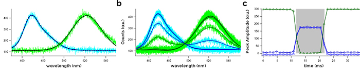
Figure 3. (a) Steady state spectra of blue and green channels with a 1.2 ms exposure time. (b) Kinetic series of 1.2 ms exposures through a 10 ms color transition. Solid lines are fits to individual spectra, resulting from a global fitting routine. (c) Peak amplitudes plotted as a function of time. Grey box marks the 10 ms color transition.
A time series of spectra was then acquired for 1 second to capture the color transition, which lasted for 10 ms. Spectra are shown for a 35 ms window bracketing this color change. These spectra were globally fit to quantify the change in peak amplitude as a function of time (Figure 3b). For this fitting routine three Gaussian line widths were used with each peak center and width held constant across all spectra. Held fit parameters were informed by the results of the steady state spectra. Only the peak amplitudes were allowed to vary without constraints. The resulting amplitudes of each Gaussian were then plotted as a function of time (Figure 3c).
As the color transition approaches, the amplitude of green channel suddenly drops to zero while the two amplitudes characterizing the blue channel simultaneously rise. For the duration of this color change (shown by the grey box) these amplitudes are constant until the color change reverses. At the edges of the color change there are spectra that contain intensity from both the blue and green color channels. LEDs turn on/off at sub-microsecond rates. So, spectra containing contributions from both color channels were simply exposing during that change. With the 1.238 ms cycle time, 7 spectra were able to be recorded of the 10 ms color change with two additional spectra exposing during the LED color transition.
To push the sCMOS camera faster, and sub-millisecond in its exposure time, we shrank the ROI height to reduce the number of pixels requiring readout. Under a reduced ROI of 2048 x 50 pixels the exposure time was lowered to 470 µs. When including the time required to readout the sensor the total cycle time becomes 499 µs, just under half a millisecond. Characterizing the steady state emission of blue and green color channels under these acquisition parameters finds a reduction of intensity relative to the 1.2 ms exposure, as would be expected (Figure 4a). With the reduced intensity only a single Gaussian line shape was used to characterize the blue channel, as the addition of a second Gaussian didn’t significantly improve the fit quality.
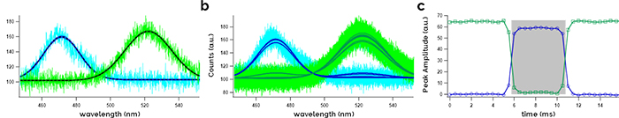
Figure 4. (a) Steady state spectra of blue and green channels with a 470 µs exposure time. (b) Kinetic series of 470 µs exposures through a 5 ms color transition. Solid lines are fits to individual spectra, resulting from a global fitting routine. (c) Peak amplitudes plotted as a function of time. Grey box marks the 5 ms color transition.
A similar time series was measured as above. A series of spectra was acquired over one second using the new exposure conditions in order to capture a single, 5 ms, green to blue color transition. Spectra across a 16 ms window, including the color change, were globally fit (Figure 4b). Using two Gaussian line shapes for these fits, the peak center and width were held constant across all spectra and only the peak amplitudes were allowed to vary. These amplitudes were then plotted as a function of time (Figure 4c).
Just before 6 ms in the time series a change in LED color is detected. As before, spectra on the edges of this 5 ms window are exposing during the color transition and contain contributions from both color channels. A total of 10 spectra were able to be recorded during the 5 ms window of time the blue channel was turned on. This is consistent with the 499 µs cycle time and demonstrates the sCMOS cameras capability of sampling the LED color with sub-ms time resolution.
A final set of experiments were performed to further highlight the application of the ZL41 Wave for fast spectroscopy with sub-millisecond time resolution. The ROI was further limited to 2048 x 8 pixels, the minimum ROI height for the ZL41 Wave. The exposure time was set to 86 µs, leading to a total cycle time of 96 µs. Under these camera settings there are ~ 10 exposures per millisecond. Despite the short exposure times, the intensity of each color channel could still be resolved (Figure 5a). These steady state spectra were each characterized using a single Gaussian line shape.
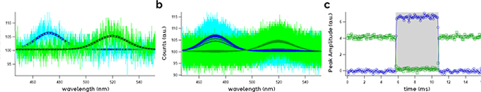
Figure 5. (a) Steady state spectra of blue and green channels with a 86 µs exposure time. (b) Kinetic series of 86 µs exposures through a 5 ms color transition. Solid lines are fits to individual spectra, resulting from a global fitting routine. (c) Peak amplitudes plotted as a function of time. Grey box marks the 5 ms color transition.
A time series was acquired for 1 second, capturing a single 5 ms color transition. Spectra from a 16 ms window surrounding this green to blue color change are shown in Figure 5b and were globally fit. Same as before, the peak centers and widths were held constant and the peak amplitudes were allowed to vary. Plotting the peak amplitudes as a function of time allows the spectral change of the LED to be easily observed (Figure 5c). A total of 52 spectra were acquired during this 5 ms period, a five-fold increase over the previous exposure conditions. While the timing of the color changes wasn’t changed the sampling rate was, providing finer temporal resolution of the color change.
In this application note we have demonstrated the application of the ZL41 Wave sCMOS cameras towards the spectroscopy of dynamic systems and show it is possible to achieve sub-millisecond time resolution. The demonstration exhibits how the technology already exists to measure broad spectral regions at frame rates exceeding 1 kHz.
For this demonstration a LED’s emission was characterized during a green to blue color transition lasting several milliseconds. Three different time series using a 1219 µs, 470 µs, and 86 µs exposure time show how it is possible to monitor transient phenomena with temporal resolution down to sub-millisecond time steps. While the experimental system in this demonstration is a simple RGB LED, this illustration can be abstracted to many spectroscopic set ups. At the frame rates relevant to these experiments (500 – >10,000 Hz) the most significant consideration will be the photon flux on these time scales to ensure there is sufficient light for a detectable signal in any given experiment.
While this application note focused on taking advantage of a sCMOS camera’s capacity for higher acquisition speeds, there are additional benefits to sCMOS camera technology that can be leveraged for spectroscopy applications. These include front-illuminated options, electronic shuttering, and the sCMOS readout architecture that can provide benefits for NIR spectroscopy, spectral imaging applications, and spectroscopies requiring a high dynamic range. Readers are encouraged to further explore the Andor Learning Center and relevant publications for…

© Oxford Instruments 2026