Drift and Drift Correction in Time-Lapse Microscopy

Microscopes are subject to thermal and mechanical drift over periods of minutes to hours. This drift primarily affects the focus, but can also impact the XY stage coordinates and is the result of various internal and external factors. Because depth of focus of the microscope is an inverse function of objective numerical aperture (NA), this problem is worst for high resolution lenses, commonly used for live cell imaging.

One way of reducing drift is to carefully control temperature in the laboratory and allow the microscope to achieve thermal equilibrium before starting time-lapse experiments. For high-end motorized inverted microscopes, manufacturers provide sophisticated closed loop solutions for focus drift correction (FDC), based on tracking the reflected light from the interface between the cover-glass and specimen. In oil immersion lenses, the reflection arises due to the difference in refractive index between the oil-cover-glass and aqueous support buffer typically used for live cells. However, this adds significant expense and is not commonly available for upright microscopes. Although a few third-party retrofit solutions are available for upright microscopes, their performance is often unreliable in situations where a range of different objectives are needed. When budget or configuration precludes the use of FDC, thermal stability combined with software correction can be used with 3D time-lapse imaging.

Practical Considerations

Temperature control in a well-designed and managed laboratory is typically around ±1 Celsius. When a microscope reaches thermal equilibrium in this environment, we find in practice that drift is in the order of 2-3 micrometers over a 12-hour time lapse experiment. If the temperature is not regulated to these stringent standards drift will increase significantly beyond this level.

To compensate for the drift in a 3D time-lapse acquisition, the acquisition protocol must take into account the drift and ensure that the focus range sampled, exceeds the specimen sampling by a factor dependent on the drift at either end of the focus sampling range. So a 10µm stack in our “well-designed scenario” would need to be increased to at least 12µm. This allows focus drift to be corrected in the drift range, with appropriate software algorithms. The increased sampling has some consequences for specimen longevity and bleaching as the specimen is exposed to 20% more illumination than in a drift-free or FDC situation. However, the correction allows for improved quantification and tracking of cells in 3D.

Algorithms

Software algorithms for correction, generally rely on correlation between adjacent time points in a 3D (volumetric) time series. The underlying assumption is that the sample will be changing relatively slowly between time points, and that a high degree of correlation in the 3D volumes will deliver a focus offset estimate, which can be applied to the subsequent volume. This process is repeated pairwise through the time series.

In some situations, users will seed the specimen cover glass with fluorescent beads, to act as fiducial (fixed reference) features. If fiducials are used, they can be segmented and tracked. The track displacements can be used for correction instead of whole image correlation, which can be a heavy computational load. Imaris utilizes tracking of fiducials for its drift correction, which is available in the Tracking Module. We will illustrate its use in later sections of this document.

An innovative, fast correlation-based algorithm known as Fast4DReg was recently published and is available in ImageJ or Fiji. (https://github.com/guijacquemet/Fast4DReg). In this algorithm correlation matching is exploited, but instead of working with the raw voxel data, the algorithm uses maximum intensity projections in 3 orthogonal axes (XYZ) before 2D correlation to estimate the offset in XYZ for each volume pair. This turns out to be very effective and an article explaining the algorithm and its application was presented in Journal of Cell Science earlier this year (J Cell Sci (2023) 136 (4): jcs260728). Since Fiji (with Bioformats) is capable of reading native Fusion/Imaris files, Fast4DReg can be used on Fusion time lapse data quite conveniently.

Illustrated Workflow 1

Imaris with fiducials -
Step 1 in this case we have a 3D time series with only fiducials (500 nm beads) in the green channel. Open the file in Imaris 10.0.

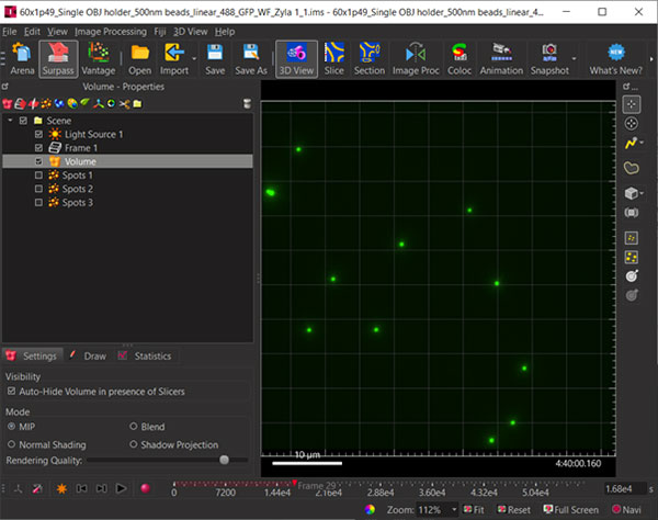
Figure 1: Load a 3D time lapse data set with fiducials.

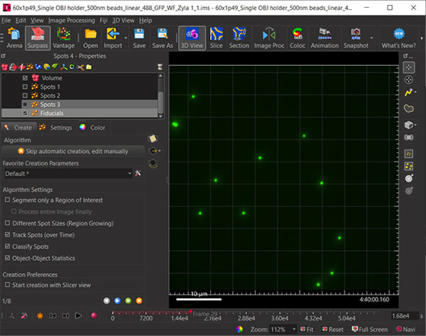
Figure 2: Create a New Spots Object and name it Fiducials. Before Spots segmentation, ensure “Track Spots” is checked. The track displacements will be used to correct the voxel data drift.

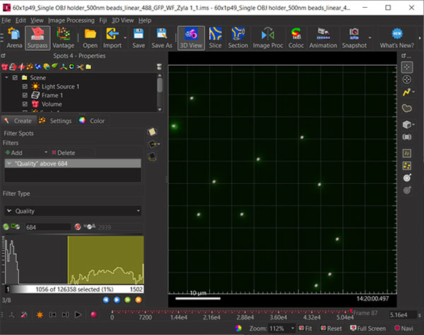
Figure 3: Use the Quality and time sliders to ensure the beads are selected across all time points. Objects are shown above as grey spheres – note the Time slider (bottom of dialog) is far to the right indicating later time points.

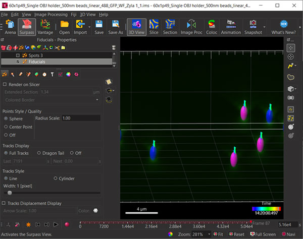
Figure 4: Once the tracks are created through the wizard you can visualize the segmented fiducials and overlay the tracks or parts thereof.

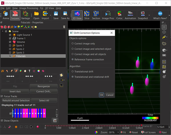
Figure 5: Select the 4th button from the left of the Spots toolbar (red circle) to reveal the Correct Drift options.

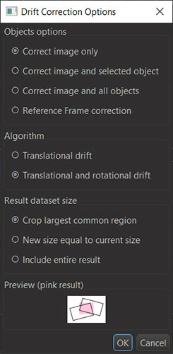
Figure 6: When the fiducials have been identified and tracked through time (Tracks), you will be able to use the Tracks to corrected the drift in the image (voxel) data with various options as shown in the dialog. You should include the image to correct your raw data.

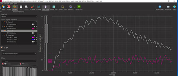
Figure 7: You can use Imaris Vantage to compare corrected and uncorrected Tracks to show the drift before and after correction. Above you will see the total drift was reduced from 2.5µm over the acquisition to 0.5µm.

Illustrated Workflow 2

Fiji and Fast4Dreg – no fiducials are required.
Refer to the Github page to access the Fast4Dreg plugin and instructions. The instructions are very clear. Open your image in Fiji (with Bioformats IMS can be read directly).

Figure 8: Visit the Fast4DReg Githib pages and follow instructions to download and install the code.

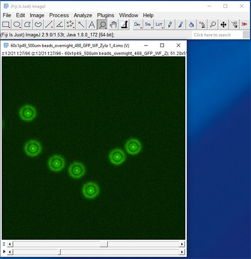
Figure 9: Load the IMS data set into Fiji - this 4D data set is the same example used in the Imaris Workflow.

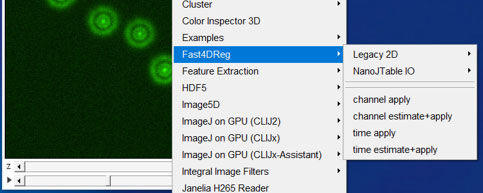
Figure 10: For this 4D data set, simply run the "time estimate + apply" script from the Plugins menu and the following dialog will be shown.

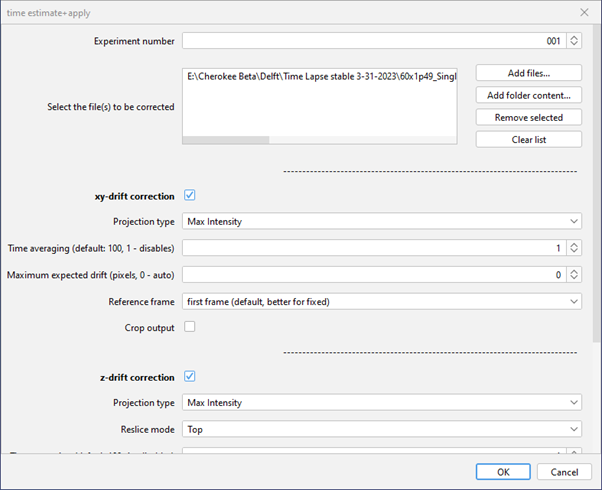
Figure 11: The Fast4DReg dialog allows you to setup batch processing options, enable XY and Z options and define various settings to speed up the process or average the estimated drfit over multiple frames and so forth.

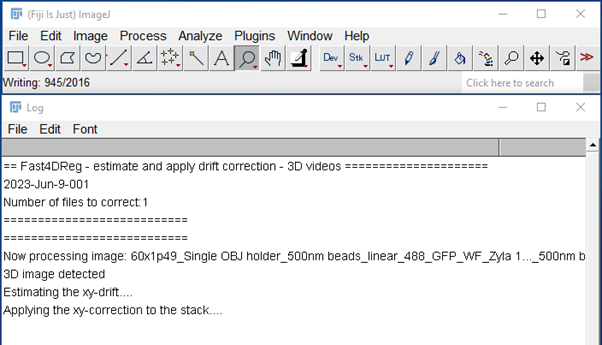
Figure 12: When the processing starts, the above status dialog is shown and the Fiji toolbar shows progress through the data set.

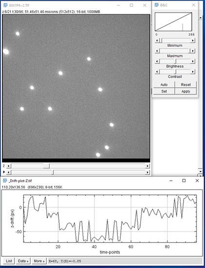
Figure 13: When the processing is complete (several to many minutes depending on data size) the results are saved in TIF format, and XY and Z drift plots are saved in TIF file graphics. Above we see the corrected 4D data set and estimated Z drift vs time.

Conclusion

Focus and lateral drift are common artefacts in timelapse imaging of live specimens. Although some microscopes have optional hardware drift correction solutions, these can be costly for inverted microscopes and simply not available for upright instruments. Fortunately, algorithmic solutions can be applied and we have annotated two approaches. The first approach uses fiducials (usually fluorescent beads) which can be segmented, tracked over time and then used for correction of voxel data using the Imaris Tracking module. The second approach is based on a fast correlation technique, known as Fast4Dreg which is freely available in Fiji or ImageJ. Fast4Dreg does not require fiducials but estimates drift between time points using correlation of maximum intensity projections (MIPs) in X, Y and Z dimensions. Both methods have their advantages and use will depend on specific user requirements and situation.