Resources
 Part of the Oxford Instruments Group
Expand
Collapse
Part of the Oxford Instruments Group
Technical Article
Author: Andrew P. Carpenter
Published: 01 Feb 2025 · Last updated: 04 Mar 2025
Intensified cameras are a class of scientific cameras for imaging and spectroscopy that possess nanosecond time/shuttering resolution while also providing single photon sensitivity. Oxford Instruments Andor’s iStar CCD and iStar sCMOS are two such examples of intensified camera technology. Herein we review the anatomy of a camera intensifier, which provides both temporal resolution and signal gain, and navigate how to optimize the intensifier settings for improved experimental results and avoid image artifacts. Additional technical notes of intensified cameras can be found in the Learning Center.1,2
The intensifier sits in front of a CCD or sCMOS camera sensor to provide the nanosecond gating and signal amplification functionalities. Briefly, an intensifier is constructed with a photocathode, a microchannel plate (MCP), and a phosphor (Figure 1). As light falls on the intensifier it first passes through the entrance window and is absorbed by the photocathode, generating photoelectrons. An important quality of the photocathode is its quantum efficiency that, much like a camera sensor, dictates the probability a photon generates a photoelectron at a given wavelength. The photoelectrons generated by the photocathode are directed towards the MCP where they can be multiplied within via a process called impact ionization. The photoelectron cloud exiting the MCP is directed towards a phosphor screen, which converts the electrons back to photons that are then imaged onto the CCD or sCMOS sensor. In Andor intensified cameras a fiber optic plate is used to couple the phosphor to the camera sensor. A fiber optic coupler is chosen over a lens coupled system in order to maximize light throughput and allow for a compact design.
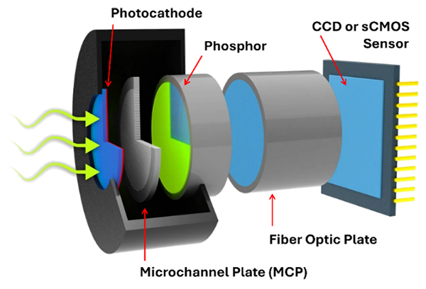
Figure 1.Illustration of a camera intensifier and its internal components.
The important properties of the intensifier come from this intensifier anatomy. Nanosecond gating capabilities arise from the ability to quickly vary the electric field between the photocathode and MCP, allowing photoelectrons generated at the photocathode to either be “rejected” or “accepted”. This gating function allows the rejection of unwanted signal outside the gate window. Impact ionization within the MCP provides the camera’s gain mechanism that multiplies weak signals, even single photons, above the camera sensor’s noise floor. While increased gain will lead to increased signal, users need to be wise with how much gain is applied otherwise they risk operating the camera in a non-optimal manner for their experiments.
A quick note on gain quantification before we proceed. When setting your gain on an Andor iStar CCD or iStar sCMOS, the gain is expressed in Digital-Analogue Converter steps ranging from 0-4095 and not absolute gain values. To determine the absolute gain value, versus the MCP DAC setting, scientific intensified cameras provide users with a camera specific measured relative gain map and conversion factors unique to the sensor acquisition parameters. These values are provided in every iStar camera’s performance sheet generated during the QC process. With these values users can calculate the photoelectrons generated at the photocathode from the counts displayed in an image (or spectrum).
Towards the goal of optimizing our intensified camera, we start by considering the phosphor inside the intensifier unit. This is chosen at the point of sale and cannot be changed afterwards. The phosphor is an important consideration as it will impact the amount of gain that needs to be applied in certain scenarios. Andor provides either the P43 or P46 phosphor. The primary difference between these two phosphors is their relative power efficiency and their decay time (to 10% peak intensity). These are summarized in Table 1 below. An appropriate way to think about the trade-off between phosphors is if you are triggering the intensifier faster that ~400 Hz, then you will need the P46 phosphor for its faster decay. Otherwise, a ghost image artifact can appear in subsequent images (or spectra) without the faster decay. However, the choice of the P46 comes at the expense of the power efficiency. This reduction in power efficiency will result in the need to apply additional gain to achieve a similar SNR to the P43, which could affect the dynamic range and linearity for a given experiment.
| Phosphor | Decay time to 10% | Relative Power Efficiency |
| P43 | ~2 ms | 1 |
| P46 | ~200 – 400 ns | 0.3 |
Table 1. Decay time and relative power efficiency for intensifier phosphors provided by Oxford Instruments Andor.
Having considered the phosphor, we turn to the relationship between MCP gain and an intensified camera’s dynamic range. Dynamic range is defined to be the ratio between the pixel well depth and the noise floor. Practically speaking, this is the ratio between the maximum and minimum detectable signals. As more gain is applied you can expect the dynamic range to shrink. It isn’t that the CCD or sCMOS sensors dynamic range is changing, but rather the signal multiplication reduces the number of incident photons that can be detected before the camera’s pixels are saturated (illustrated in Figure 2a).
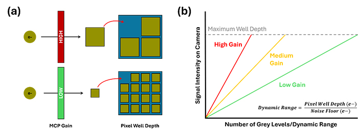
Figure 2. (a) Representation of the effect of MCP gain on the dynamic range of a camera sensor. As photoelectrons are amplified within the MCP, only so many amplified “pieces” can be accommodated by the pixel’s well depth. (b) Generalized illustration of how increases in MCP gain lead reductions in the dynamic range.
Consider, as an example, the limit of a single photon. If significant gain is applied, the single photoelectron generated at the photocathode will be multiplied into a large electron cloud by the MCP. This will be converted into many photons by the phosphor and detected as an intense signal by the camera sensor. Under these operating conditions (high gain) the intensifier has enabled the detection of a single photon, but the number of photons that can be detected is few. The important observation to make is that as the MCP gain increases the camera sensor’s well depth will be filled by fewer incident photons on the photocathode (Figure 2b). Thus, resolving significantly different signal levels across an image (or spectrum) can become difficult under high gain conditions.
When optimizing MCP gain consider only using as much gain as necessary to overcome the camera noise floor, with a general rule being to only apply 5-6x more gain than what is necessary to just overcome the noise floor. For instance, if a pixel has 2e- readout noise, the MCP gain that would offer a balance between overcoming the noise floor and protecting the dynamic range would be 2e- x 6 = 12. If using an intensified sCMOS camera, a 4x4 bin of pixels would increase the read noise 2e- x SQRT(16) = 8e-, leading to a best compromise MCP gain setting of 8e- x 6 = 48. Note, this 5-6x gain is not the DAC gain setting, but is the gain that would be calculated from the relative gain map and acquisition parameters reported in the performance sheet.
The exception to this guideline is if you are using an intensified camera for photon counting applications. In this case, set the MCP gain to its maximum to provide for the best discrimination of photons above the background.
Important to many imaging and spectroscopy applications is the linear response of the camera. With an intensified camera the linearity will depend on the phosphor output that is imaged onto the CCD or sCMOS sensor. Just as with dynamic range, the intensifier’s linearity will be dependent on your gain level. Figure 3 is representative of a phosphor’s emission as a function of the photocathode’s illumination. For a fixed gain setting, as the intensity of light on the photocathode increases the emission of the phosphor increases. This is good, as increases in photons at the photocathode should correspond to increases in phosphor emission that will be sent to the camera sensor. However, the exact relationship between photocathode illumination and phosphor emission will vary depending on MCP gain.
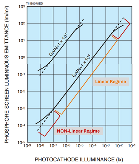
Figure 3. Characteristic plot of phosphor emission as a function of photocathode illuminance.3 Linear (orange) and non-linear (red) regions are highlighted for the gain = 104 curve.
Focusing on the 104 gain curve, the phosphor response is linear for a broad range of photocathode illuminance but turns nonlinear at low and high illuminance. As the gain is increased to 107 the linear response regime shrinks and the nonlinear response regime grow. Recall that the phosphor is responding to the amplified photoelectron signal coming from the MCP. So, with increases in gain come increases in the number of MCP generated photoelectrons and the phosphor can be saturated even though the number of photons on the photocathode remains low.
If you are working with an intensifier containing a P46 phosphor, the amount of gain you need to apply can increase relative to an identical measurement using a P43 phosphor. Under identical illuminance and gain conditions the number of photoelectrons will be the same before the phosphor, but the number of photons generated by the P46 phosphor is lower as a consequence of the P46’s lower relative power efficiency. Therefore, considering your MCP gain becomes even more important when optimizing the linearity of your intensifier response if using the P46 phosphor since the linearity for an intensifier with the P46 phosphor can be reduced relative to the P43.
An additional feature of Andor intensified cameras that is worth mentioning is the Anti-Brightness Control (ABC). This is a camera functionality that monitors the phosphor current to minimize the risk of phosphor damage at high currents. If the phosphor current exceeds a certain threshold (i.e. too many photoelectrons hitting the phosphor) the voltage governing MCP gain will be lowered, automatically, to reduce the risk of phosphor damage. When working with high gain, or bright signals, the ABC has the potential to impact the perception of the camera’s linearity.
The advice here is the same as that for optimizing dynamic range – keep MCP gain as low as possible to access a larger linear response region. This becomes even more important when working with an intensified camera containing a P46 phosphor.
Having considered the importance of optimizing MCP gain for dynamic range and linearity, we now turn to perform a séance to understand and prevent “ghost” artifacts from appearing in our images. In the context of this technical note ghost artifacts are defined as contributions to an image that are affected by the previously acquired image and not the ghost imaging experiments that seek to understand the quantum nature of our world. 4,5 Ghost artifacts can contribute positively or negatively to images (Figure 4) and the underlying mechanisms for these contributions differ.
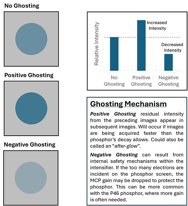
Figure 4. Cartoon illustration and mechanisms behind positive and negative ghost imaging. The “No Ghosting” image represents a measurement without artifacts, while the “Positive Ghosting” and “Negative Ghosting” represent images with ghost artifacts.
Positive ghosting is a phenomenon where additional light intensity from the previous frame reaches the CCD or sCMOS sensor during a subsequent image. This is the result of a phosphor response not being fully decayed, either by attempting to acquire frames faster than the phosphor decay or by a long-lived emission from the phosphor under bright conditions. To eliminate positive ghosting the number of photoelectrons falling on the phosphor needs to be reduced by reducing the MCP gain or more time between frames to allow the phosphor to fully decay.
Negative ghosting is the opposite phenomenon, where light intensity appears to be missing from the image. In this scenario, presuming nothing about the sample or illumination source has changed, an internal safety mechanism has been triggered that works to protect the phosphor from damage. This is the aforementioned Anti-Brightness Control. In Andor’s intensified cameras the ABC will activate when the camera detects the phosphor is approaching a damage threshold and will drop the gain across the MCP for subsequent images to protect the phoshor. Resolving negative ghosting requires a reduction in gain.
To avoid the appearance of ghost artifacts, pay attention to the triggering rate of your intensifier and the gain you are applying. If you are triggering faster than the decay time of the phosphor, you might experience positive ghost artifacts. If you have the gain set to high you may trigger the ABC safety mechanism, resulting in an automatic reduction in gain and drop in signal levels relative to previous frames. Thus, similar to optimizing for dynamic range and intensifier linearity, increase the MCP gain only as high as needed and no higher.
With all the attention given to optimizing gain it would be natural for the question to emerge – “How do I optimize gain in the beginning?” At the most basic level, the best practice is going to be to not over-illuminate and potentially damage the intensifier. In what follows we describe one way to establish the appropriate gain parameters, though other procedures may exist.
1. Before attempting any measurements, identify a standard sample you know will provide signal and estimate the amount of signal you would expect on a bare camera sensor. This should roughly (within an order of magnitude) be what is seen with no additional gain applied.
2. Setting up for the first measurement, start with a lower gain and higher gate width than you plan to use during your experiments. If you are using an external trigger you can estimate your gate delay by considering the length of your trigger cable and the injection delay of the camera. Set your gate delay and use a wide gate width to make sure you capture your optical signal.
3. For the first measurement the goal is to check whether your camera saturates at the lowest exposure time. A quick tip – When working within Solis, type “0” and hit enter into the exposure time box and it will auto-populate with the lowest possible exposure time for your camera under its current acquisition settings.
4. If you do not detect a signal under these conditions, progressively take away ND filters and increase the exposure time until there are no more ND filters and you have reached the exposure time of your typical planned experiments. If you still are unable to measure a signal at this point, slowly increase the gain until your signal appears.
5. Once you have a signal, sequentially optimize the gain as you remove all ND filters and approach your experiments’ exposure times. Converge on the amount of gain that is 5-6x what is necessary to just overcome the noise floor.
6. Lastly, progressively reduce your gate width while optimizing the gate delay until you are at the gate settings that will be used in your experiments. Verify the gain being applied is still appropriate for the new gate settings. Update the gain setting if necessary.
Following this general outline, one should be able to converge on an appropriate gain level that will maximize dynamic range and linearity, while keeping the intensifier safe from damage and avoiding any image (spectral) artifacts.
While every researcher’s experimental set up will be different, everyone should mind the gain they apply. Because the intensifiers in front of iStar CCD and iStar sCMOS cameras are the same, both camera families can be susceptible to issues surrounding high gain (reduced dynamic range, non-linearities, ghost artifacts). This is particularly important when you are working with a P46 phosphor, where higher gain may be needed to compensate for the lower relative power efficiency. If you are using an intensified sCMOS the camera could be more susceptible to issues arising from fast frame rates due to the faster read out speed of the sCMOS sensor. If you are performing kHz spectral measurements or PIV imaging experiments6, the short time between frames makes one more susceptible to issues of negative and positive ghosting.
Best practice would suggest using a standard sample that mimics routine experiments to allow one to determine the appropriate MCP gain for best dynamic range and linearity. This will also help circumvent ghost artifacts, avoid non-linearities, and maximize your dynamic range.

© Oxford Instruments 2026