Optical Coherence Tomography (OCT) is a powerful imaging technique used routinely by clinicians to aid in the diagnosis and monitoring of a range of diseases and medical conditions. Imaging the layers of the retina in the eye is the main area of usage but it is also standard for imaging the cornea. It has also been developed and used to varying degrees in areas such the diagnosis of skin conditions, dentistry, and endoscopic imaging of the cardiovascular and gastro-intestinal systems [1, 2, 3, 4]. Outside of medicine it is becoming routinely used in areas such as industrial non-destructive testing [5], and art and historical artefact examination [6].
OCT can provide high resolution images in 2D and 3D of the layers of tissue in-vivo. This case note describes the work of a multi-disciplinary group at Liverpool University who are developing a new generation of ophthalmic instrument based on a technique known as Line Field – Optical Coherence Tomography (LF-OCT) [7]. This approach offers a number of key benefits over current clinically approved instruments including the simultaneous acquisition of complete 2D sectional images or ‘B’ scans, high data acquisition speeds, ultrahigh sensitivity and spatial resolution.
Introduction
Optical Coherence Tomography (OCT) is the optical analogue of ultrasound and it allows for cross-sectional imaging of materials that are partially transparent to light signals. It operates by measuring the 3D location of light scattering and reflections, from scattering particles and interfaces where there are changes in optical refractive indices respectively [8]. Low coherence interferometry between a reference beam and the reflected signal beam is used to measure and differentiate the time delay, thus depth, of the many tiny reflections. The ranging of these signals by low coherence interferometry can be done using just a spectrometer to measure the monochromatic interference amplitude of each measured wavelength of light and then exploiting their combined Fourier mathematical properties. The lateral (sideways) locations of the reflections are found with the same basic principles of a camera. Figure 1 shows a schematic of an incident pulse interacting with the layers of the eye retina.
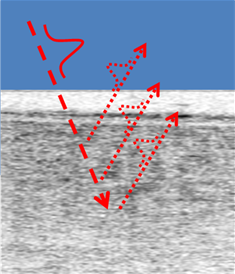
Figure 1: OCT image of the layers in the cornea of the eye [7].
Most modern OCT systems only measure one lateral position at a time. The Liverpool group are using an alternative ‘Line Field’ approach, which measures all the lateral positions in cross-sectional image simultaneously, to image the cellular layers of the cornea and tear film, with a view to better understanding a range of diseases of the cornea such as corneal ulceration, Fuchs dystrophy, and refractive disorders [9]. Significant benefits should be realised for patients with the improved speeds and high resolution of LF-OCT.
At the heart of any OCT system is an interferometer, which is based on the same principals as the Michelson interferometer of the famous Michelson-Morley experiment and the modern gigantic instruments used to measure gravitational waves. The particular type of interferometer used in the first Liverpool prototype is of the Linnik design [10]. This has identical optics in the reference and sample arms of the interferometer, which means the relative time differences that light of different wavelengths takes to travel through an object (i.e. the optics) are matched in both arms of the interferometer and has no impact on the interference signal. Without this matching, the mismatch of time differences between the different wavelengths of light (dispersion) blurs the ranging of the signals. The distinct benefit for the Liverpool system is the achievement of ultra-high (2.1 μm in air) depth resolution without the need for physical or data manipulation in the system.
Some background - Different approaches to OCT
OCT developed from techniques such as low-coherence interferometry [11], and femtosecond optical ranging [12], with the terminology and development of the first widely used technique emerging in the early 90’s [13]. Since then there have been multiple variants and developments of the basic technique [14, 15]. The large amount of OCT variants comes from the fact that there are several methods to achieve depth ranging (Time Domain, Swept Source and Spectral Domain), several methods to get lateral information (scanning point, line field and full field), a number of functionalities which can be built in (e.g. polarisation sensitivity, OCT angiography and OCE), physical construction of interferometer (e.g. fibre Michelson, fibre Mach-Zander, free space Michelson, Linnik and common path) and where physically you implement your OCT sensor (e.g. on the end of an endoscope in endoscopic OCT). These different options can be put together in a multitude of combinations. LF-OCT is among the more recent developments. Figure 2 shows the relationship between the main variants of the base approach including the common acronyms used.
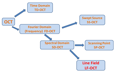
Figure 2: The main variants of the OCT imaging technique
The original approach was based on Time Domain (TD) measurements but this has now been superseded by Fourier Domain (FD) methods. Fourier Domain or FD-OCT can be distinguished into two main sub-groupings depending on whether a tunable light source (i.e. a tuneable wavelength output laser) is used to present a series of individual wavelengths sequentially in the measurement or if all the wavelengths (from a broadband source) are presented simultaneously and a spectrometer or spectrograph is used to capture the dispersed spectra. The former method is referred to as Swept Source (SS) and the latter as Spectral Domain (SD).
In the common scanning point implementation of SS-OCT, a very fast single point detector is then used to measure the interference signal. This sequentialisation approach does give benefits in terms of image depth, speed and SNR but the limited optical bandwidth of source sweeping ranges means low depth resolution. Scanning point SD systems use a single channel input spectrometer with a dispersion element such as a grating to produce a single spectrum which is captured on a 1D-line detector such as a photodiode array or CCD. In this case all the wavelengths from the broadband source illuminate the sample or tissue at the same time. Currently most standard clinical products are based on Scanning Point SS and SD systems, where the light illumination is focused to a point on the sample resulting in a single channel depth profile at that single point – which is referred to as an ‘A’ scan (a term borrowed from ultrasound imaging). To build up a 2D sectional image through the tissue sample, as illustrated in figure 1, the point of illumination has to be scanned laterally across the sample. The resulting 2D dataset is referred to as a ‘B’ scan image. This can be extended by doing further raster scanning (or a series of parallel scans) across the sample to build up a 3D imaging data volume.
Line Field OCT takes an increased parallelisation approach compared to the well-established scanning point method. A line of illumination is delivered on to the sample and the reflected signal is subsequently focused on the entrance slit of a multi-channel imaging spectrograph, which then measures the spectral interferograms of all positions at the same time. This allows for the illumination of one complete section through the sample resulting in the capture of one complete ‘B’ scan image in one acquisition. Essentially all the spectral information from each point along the line on the sample is captured in parallel – analogous to hyperspectral or high density multi-track spectral imaging. Parallel acquisition of A-scan data leads to much faster acquisition times. This has an advantage of reducing artefacts caused by motion for example when the patient’s heart beats or they breathe.
Spatial resolution in both the lateral and axial (depth into the tissue) is of key importance in OCT measurements. The axial resolution depends intrinsically on the optical bandwidth of the light source used. On the other hand the lateral resolution is generally determined by the spot size of the light beam or confocal pinhole aperture used in the optical path for point scanning systems. In the case of LF-OCT the lateral resolution will depend intimately on the imaging quality of the spectrograph used. With the possibility of high axial resolutions OCT is proving to be an ideal tool for in-vivo imaging through relatively thick (several mm) sections of biological issue.
The main characterising features, including advantages, for OCT based imaging are summarised in Table 1.
| Table 1: Main Aspects of Conventional OCT |
| Non-invasive diagnostic technique for imaging |
| Optical analogue of Ultrasound imaging |
| In-vivo and in-vitro sectional views |
| Morphology of sample |
| Uses interference of optical light (visible and NIR) |
| Axial (depth) resolution typically ~10 µm |
| Lateral (transverse) resolution typically ~20-50 µm |
| Penetration depth into tissue typically ~3 mm |
| High sensitivity (and Dynamic Range) |
| Real-time as well as standard imaging |
| Does not require physical contact |
| Relatively safe optical biopsies possible |
A more detailed look at Liverpool LF-OCT system
The LF-OCT setup at Liverpool is based on a Spectral Domain (SD) arrangement where an Andor Shamrock 303i imaging spectrograph is used to measure the spectral interferograms for all A-Scans simultaneously. The light source is an ultra-broadband Super-Continuum (SC) laser. High and low pass filters were used to define the used optical band from 700 nm to 1000 nm. To achieve the ‘Line Field’ geometry a cylindrical lens and an objective were used to form the illumination beam into a line focus on the sample.
This illumination pattern enabled a complete B-scan to be acquired at the same time in contrast to the scanning point (SP) approach where multiple A-scans have to be acquired to build up the equivalent of the B-scan. The line image from the sample was imaged on to and aligned with the entrance slit of the spectrograph. A schematic layout of the experimental setup is shown in figure 3. As a first phase in the ‘proof of concept’ and development of an instrument, the group used off-the-shelf instruments which included an Andor Shamrock 303i spectrograph, a CCD camera and a Neo sCMOS camera.
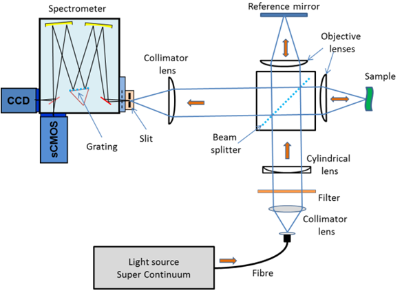
Figure 3: Schematic of experimental arrangement.
A 300 g/mm grating and toroidal optics in the Shamrock spectrograph dispersed the interfered light at the spectrograph slit into multiple spectral interferograms across the output focal plane. These interferograms were captured on the 2D CCD or sCMOS detectors depending on which detector was being used at a given time. This spectral arrangement is analogous to high-density multitrack spectral or indeed hyperspectral imaging. Like these arrangements, the spatial resolution of these channels or tracks is dependent on the imaging quality of the spectrograph. An sCMOS Neo camera on the direct exit port camera was used for high-speed imaging and a slower back illuminated (BI) CCD camera on the side exit port was used for high-resolution imaging. A software application developed in Matlab using the Andor SDKs for the spectrograph and cameras allowed for automated control of the system and the real-time display of OCT images.
Some Results [16]
![OCT images of a donor human cornea ex-vivo taken with two current commercial systems (SP-SS left, SP-SD middle) and Liverpool’s LF-OCT system (right). The ultra-high axial resolution of the system means that all 5 layers of the cornea and details of the stroma are better resolved than the current commercial systems [16].](https://www.oxinst.com/learning/uploads/inline-images/lf-oct-04-20180904091938.png)
Figure 4: OCT images of a donor human cornea ex-vivo taken with two current commercial systems (SP-SS left, SP-SD middle) and Liverpool’s LF-OCT system (right). The ultra-high axial resolution of the system means that all 5 layers of the cornea and details of the stroma are better resolved than the current commercial systems [16].
Ultra-high resolution was possible with their prototype instrument. A comparison of sectional views through the layers of cornea tissue acquired by different instruments is shown in figure 4. The image from the Liverpool system is shown on the right and is compared with images from two current commercial systems. These sectional images or ‘B’ scans illustrate the fine structure within the human cornea. This image is derived from measurements where the light is incident from the top and the image shows layers within the tissue in the axial direction down into the tissue; this explains in part the reduction in contrast towards deeper layers due to the attenuation of the light as it propagates into and out of the sample. Clearly the resolution and clarity for the image on the right is notably better as evidenced by the clearer visibility of the fine structure within the tissue. Operating in the conventional quasi-CW mode the group were able to achieve axial resolutions down to 2.1 mm, and lateral resolutions of 18 mm.
When running the Neo camera at 100 full frames/s, 3D volume imaging speeds up to 213 kA-Scans per second were achievable representing a very large increase in speed compared with current clinical instrumentation. The group are also working on a range of techniques for improving the image quality further by for example using Fourier phase analysis to handle the degradations in image quality due to artefacts [5].
Conclusion
The potential of LF-OCT for significant improvements in the performance for clinical OCT instruments has been clearly demonstrated in this work. Instrumentation incorporating fast-frame-rate and sensitive imaging cameras (e.g. Neo or Zyla) along with high fidelity imaging spectrographs (e.g. Holospec f1.8) are required for the realisation of such LF-OCT systems. Some of the advantages of LF-OCT compared with established OCT techniques are given below:
- Ultra-high axial resolution
- Reduction in motion artefacts (due to faster acquisitions)
- Higher imaging speed at lower overall illuminating point intensities (due to line focus illumination of imaged section only)
- Lower risk of damage in-vivo due to lower overall fluence.
Acknowledgement: The information and figures for this note were gratefully received from Dr S Lawman of the Dept. of Electrical Engineering and Electronics, & Dept. of Eye and Vision Science, University of Liverpool.
References
- www.octnews.org
- Sakata LM,1 DeLeon-Ortega J, Sakata V and Girkin CA, (2009) Optical coherence tomography of the retina and optic nerve – a review. Clinical and Experimental Ophthalmology 37: pp90–99
- Gambichler T, Pljakic A, Schmitz L (2015) Recent advances in clinical application of optical coherence tomography of human skin. Clinical, Cosmetic and Investigational Dermatology Vol: 8 pp345–354
- Bezerra HG, Costa MA, Guagliumi G, Rollins AR, Simon DI. (2009) Intracoronary Optical Coherence Tomography: A Comprehensive Review. J Am Coll Cardiol Intv. Vol 2(11):1035-1046.
- Lawman, S., Zhang, J., Williams, B. M., Zheng, Y., & Shen, Y. C. (2017, June). Applications of optical coherence tomography in the non-contact assessment of automotive paints. In Optical Measurement Systems for Industrial Inspection X (Vol. 10329, p. 103290J). International Society for Optics and Photonics.
- Liang, H., Peric, B., Hughes, M., Podoleanu, A., Spring, M., & Saunders, D. (2007, July). Optical coherence tomography for art conservation and archaeology. In O3A: Optics for Arts, Architecture, and Archaeology (Vol. 6618, p. 661805). International Society for Optics and Photonics.
- Lawman S, Dong Y, Williams BM, Romano V, Kaye S, Harding SP, Willoughby C, Shen Yao-Chun and Zheng Y (2016) High resolution corneal and single pulse imaging with line field spectral domain optical coherence tomography. Optics Express Vol. 24, No. 11 (12395)
- http://obel.ee.uwa.edu.au/research/fundamentals/introduction-oct/
- https://www.liverpool.ac.uk/ageing-and-chronic-disease/research-groups/oph-img-analysis/projects/ultra-sensitiveopticalcoherencetomographyoctimagingforeyedisease/
- https://en.wikipedia.org/wiki/Linnik_interferometer
- Fercher AF, Mengedoht K, Werner W (1988) Eye-length measurement by interferometry with partially coherent light. Optics Letters Vol. 13, No. 3
- Fujimoto JG, De Silvestri S, Ippen EP, Puliafito CA, Margolis R and Oseroff A (1986) Femtosecond optical ranging in biological systems. Optics Letters Vol. 11, No. 3
- Huang D, Swanson EA, Lin CP, Schuman JS, Stinson WG, Chang W, Hee MR, Flotte T, Gregory K, Puliafito CA, and Fujimoto JG (1991). Optical coherence tomography. Science 254(5035), pp1178–81
- Fercher AF, Drexler W, Hitzenberger CK and Lasser T (2003). Optical coherence tomography—Principles and Applications. Rep. Prog. Phys. 66 (2003) 239–303
- Gabriele ML, Wollstein G, Ishikawa H,Kagemann L, Xu J, Folio LS and Schuman JS(2011). Optical Coherence Tomography: History, Current Status, and Laboratory Work. Investigative Ophthalmology & Visual Science, Vol. 52, No. 5