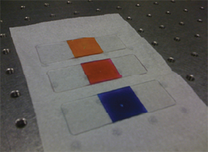
Figure 1: A digital photograph of three different concentrated dye solutions sandwiched between a glass slide and a coverslip. From top to bottom: Na-FITC (0.5 g/mL), Rose Bengal (0.3 g/mL), Acid Blue 9 (0.35 g/mL).
Written below is a simple protocol detailing a method to create a fluorescent test sample that can be used to measure the illumination uniformity of your confocal microscope (laser scanning or spinning disk). This protocol is an extension of a procedure originally developed by Michael M. Model at Kent State University involving the formation of concentrated fluorescent dye solutions [1, 2]. As a result of their large optical density, these dye solutions possess the unique property that, if sandwiched between a glass slide and a coverslip, they will only emit fluorescence from an extremely thin, planar region (diffraction-limited in the axial z-direction) immediately adjacent to the coverslip when illuminated with an appropriate excitation wavelength. Therefore, when viewed with a confocal microscope, any non-uniformities in the fluorescence image of the concentrated solution reflect the degree of non-uniformity of the illumination profile for a given set of aligned optical components in the confocal microscope (laser, filters, objective, image forming optics, pinhole(s) and detector). Different dyes can be selected for different excitation/emission wavelength combinations. These concentrated dye solutions are preferred over traditional fluorescent plastic slides for this type of measurement because the plastic slides accentuate the pinhole cross-talk effect due to their intense brightness and thier thickness that extends well beyond the focal volume.
Materials
- latex or nitrile gloves
- safety goggles
- 1 mm thick glass slides
- standard #1.5 thickness (nominal 170 mm) glass coverslips
- ethanol or isopropyl alcohol
- clear nail polish
- lens paper
- 10 mL pipette and pipette tips
- 10 mL glass/plastic test tube with stopper
- test tube vortexer/shaker
- sonicator bath
- chemical weighing balance
- distilled water
- fluorescent dyes in powder form (see table below) which can be purchased from Sigma-Aldrich
| Dye |
Excitation Wavelength |
Emission Wavelength |
Sigma-Aldrich Product code |
| Sodium-Fluorescein (Na-FITC) |
Blue (473 nm, 488 nm, 491 nm) |
Green (510 nm - 560 nm) |
F6377-100G |
| Rose Bengal |
Green(532 nm, 543 nm, 561 nm) |
Red (560 nm - 620 nm) |
198250-5G |
| Acid Blue 9 |
Red (633 nm, 642 nm) |
Deep red (650 -800 nm) |
861146-5G |
Protocol
- While wearing gloves and safety goggles, clean a single glass slide and coverslip with a few drops ethanol or isopropyl alcohol on a piece of lens paper. Gently wipe the coverslip and glass slide with the wetted paper, avoiding residual streaking.
- Weigh out 0.5 g of Na-FITC powder on the weighing balance and deposit into the test tube.
- Add 1 mL of distilled water into the test tube to yield a Na-FITC solution with a concentration of 0.5 g/mL. Cap the test tube and shake vigorously with the test tube vortexer/shaker for 10 min. The resulting solution should appear homogenous by eye. Rose Bengal and Acid Blue 9 concentrated solutions must be prepared at lower concentrations because of their lower solubility (0.3 g/mL and 0.45 g/mL respectively).
- Lower and hold the end of the test tube in the sonicator bath to a depth that matches the depth of the dye in the test tube. Sonicate the solution for 30 min. No heating of the bath is required.
- Pipette a 6 mL drop onto the cleaned glass slide. Hold the cleaned coverslip above the drop at a 45 degree angle and allow to fall on the drop causing it to spread to a thin layer between the slide and the coverslip. The exact thickness of the layer between the two glass interfaces does not matter. Let the slide-dye-coverslip sandwich sit for 10 min.
- Place the slide-dye-coverslip sandwich on the microscope stage with the coverslip side facing the objective lens. If using a water or oil immersion objective lens, place a small drop of the immersion medium on the coverslip (upright microscope) or the objective lens (inverted microscope).
- Either manually (or automatically in acquisition software) choose an excitation/emission wavelength light and filter combination that is appropriate for the dye being examined. For example, a concentrated Na-FITC solution can be excited with a 488 nm line and imaged through a standard FITC or GFP filter set (dichroic mirror and emission barrier filter).
- Set the excitation power to 50% it’s maximum power level. In the image acquisition preview/focus mode, slowly begin to focus on the concentrated dye solution which emits light at a focal depth immediately adjacent to the coverslip. Increase the detector exposure and gain (spinning disk) or voltage and gain levels (laser scanning) as needed. The dye solution’s fluorescence signal is greatest at only one focal position. Once this focal position has been roughly found, decrease the excitation power such that no pixels in the image saturate. If any obvious photobleaching is observed in preview mode, decrease the excitation power further and increase the detector sensitivity until the fluorescence signal lies near the top of the dynamic range. On a laser scanning confocal microscope, use the slowest scan speed, set the scan zoom level to 1x, the image dimensions to 512x512 pixels, and the confocal pinhole to 1 Airy unit, readjusting the detector voltage and gain if needed.
- Acquire a z-series centered on the dye solution (-10 mm to +10 mm from the current focal position), choosing a z-step of 50 nm if using a high numerical aperture (NA) immersion objective lens (water or oil) or 100 nm for a low NA, low magnification objective lens. Other appropriate objective lens z-steps can be determined online here.
- Save the z-series as a single file or as a series of images (preferably .tif format) in a directory folder.
Image Analysis
The degree of illumination uniformity can be quantified with any commercial image processing software package such as Metamorph (Molecular Devices) or ImagePro (Media Cybernetics). One can also download and use the freely available open-source image analysis program ImageJ. The instructions described below are a step-by-step guide for uniformity analysis in ImageJ, but the same general method can be applied in any of the commercial software packages as well. Alternatively, Spectral Applied Research can produce and email you a detailed report about your system’s illumination uniformity, free of charge (see instructions below for transferring data to Spectral).
- Launch ImageJ and open the saved z-series. If the z-series is saved as a single file, it can be opened using ImageJ’s File=>Open… dialog. If the z-series is saved as a sequence of images, open it using ImageJ’s File=>Import=>Image Sequence… dialog. If ImageJ does not recognize the proprietary file format of your confocal microscope manufactuerer, download and install the Bio-Formats LOCI plugin for ImageJ and use this plugin to import the file.
- Create a maximum intensity z-projection of the opened z-series by selecting the z-series window and using ImageJ’s Image=>Stacks=>Z Project command, choosing the Max Intensity option (Figure 2). Because of the small depth of field in confocal imaging, the fluorescent area produced by the concentrated dye solution immediately next to the coverslip may never appear in focus (indicating a tilt of the slide-dye-coverslip sandwich on the sample stage). Creating a z-projection image of the z-series removes any non-uniformities due to this effect [1, 2].
- Select the resulting z-projection image and draw a straight corner-to-corner (top-left to bottom right, or top-right to bottom-left) line segment using ImageJ’s straight line tool found in the main toolbar (Figure 2).
- Create a line profile graph by choosing Analyze=>Plot Profile. Click the Copy button at the bottom of this graph (Figure 2).
- Mathematically fit a parabola to this line profile using the Analyze=>Tools=>Curve Fitting command (Figure 3). A window will appear where you can paste in the numerical values of the line profile graph. Select the 2nd Degree Polynomial option from the drop down menu and click Fit. Another graph will appear where the line profile data is plotted as a series of circular points and the fitted parabola appears as a solid curve. Click the List button at the bottom of this new graph to call up a table of Plot Values for the fitted parabolic curve.
- Expand the Plot Values window, scroll through the table and find the maximum and minimum Y1 values. Record these values as MaxY1 and MinY1 respectively (Figure 3).
- The corner-to-corner %roll-off (also known as the “flatness of field”) is a simple index that can quantify the degree of uniformity of your confocal illumination profile [4]. Its value is calculated as:
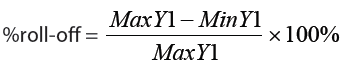
If desired, a mean value can be obtained by averaging the %roll-off values for both diagonal line profiles (top-left to bottom-right and top-right to bottom-left).
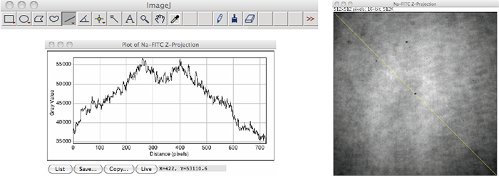
Figure 2: A Z-Projection image of a Na-FITC concentrated dye solution z-series with a drawn top-left to bottom-right line segment (left) and the corresponding line profile graph of pixel intensity values along this line (right). Image acquired with a Yokogawa CSU-X1; 491 nm excitation; 525/30 nm emission. Analysis performed with ImageJ version 1.46.
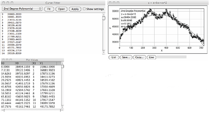
Figure 3: ImageJ’s curve fitting window tool (top left) and a resulting fitted line profile graph (top right). By clicking the List button in the graph window, a Plot values table will be called (bottom left) from which the MaxY1 and MinY1 values can be determined.
References
- Model, M.A. and J.L. Blank, Intensity calibration of a laser scanning confocal microscope based on concentrated dyes. Analytical and Quantitative Cytology and Histology, 2006. 28(5): p. 253-261.
- Model, M.A. and J.L. Blank, Concentrated dyes as a source of two-dimensional fluorescent field for characterization of a confocal microscope. Journal of Microscopy-Oxford, 2008. 229(1): p. 12-16.
- Dimas, C.F., J.J. Kuta, and M. Hubert, An enhanced method of obtaining uniform excitation radiation for fluorescence microscopy, in Applications of Photonic Technology 6 - Closing the Gap between Theory, Development, and Application, R.A. Lessard and G.A. Lampropoulos, Editors. 2003, Spie-Int Soc Optical Engineering: Bellingham. p. 558-567.
- Pawley, J., Handbook of Biological Confocal Microscopy. 3rd ed. 2006, New York: Plenum Press.
 Part of the Oxford Instruments Group